- Published on
Dự Đoán Giá Cổ Phiếu Với Mạng LSTM
- Authors
- Name
- Kevin Nguyen


Chuẩn Bị Môi Trường
Trước khi bắt đầu, hãy đảm bảo bạn đã cài đặt các thư viện cần thiết như Pandas, Matplotlib, NumPy và TensorFlow.
import pandas as pd
import matplotlib.pyplot as plt
import numpy as np
import tensorflow as tf
from tensorflow import keras
from tensorflow.keras.models import load_model
import seaborn as sns
import os
from datetime import datetime, timedelta
import warnings
warnings.filterwarnings("ignore")
plt.style.use('fivethirtyeight')
Đọc Dữ Liệu
Về dữ liệu bạn có thể sử dụng dataset
Đầu tiên, chúng ta cần đọc dữ liệu từ tệp CSV. Chúng ta sẽ sử dụng Pandas để làm việc này.
data = pd.read_csv('VIC.csv')

print(data.shape)
print(data.sample(7))
Kích thước dữ liệu: (101266, 8)

| Ticker | Date/Time        | Open | High | Low  | Close | Volume | Open Interest |
|--------|------------------|------|------|------|-------|--------|---------------|
| VIC    | 7/2/2020 9:34   | 90.3 | 90.3 | 90.3 | 90.3  | 250    | 0             |
| VIC    | 8/5/2020 13:29  | 88.0 | 88.0 | 88.0 | 88.0  | 10     | 0             |
| VIC    | 1/9/2019 9:34   | 101.4| 101.4| 100.1| 100.1 | 830    | 0             |
| VIC    | 7/6/2020 11:24  | 91.4 | 91.4 | 90.6 | 90.6  | 50     | 0             |
| VIC    | 12/28/2018 10:41| 102.5| 102.8| 102.5| 102.8 | 20     | 0             |
| VIC    | 3/11/2020 11:06 | 96.4 | 96.5 | 96.4 | 96.4  | 2980   | 0             |
| VIC    | 3/15/2019 10:14 | 118.8| 118.8| 118.7| 118.8 | 220    | 0             |
Tiền Xử Lý Dữ Liệu
Sau khi đọc dữ liệu, chúng ta cần tiền xử lý để chuẩn bị cho việc xây dựng mô hình. Các bước bao gồm chuyển đổi cột 'Date/Time' thành kiểu datetime, loại bỏ các cột không cần thiết và kiểm tra dữ liệu rỗng.
data['Date/Time'] = pd.to_datetime(data['Date/Time'])
data.info()
data = data.drop(['Open Interest'], axis=1)
data.info()
data.isnull().sum()
Trực Quan Hóa Dữ Liệu
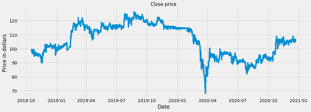
Trước khi xây dựng mô hình, chúng ta nên hiểu rõ dữ liệu bằng cách trực quan hóa nó. Dưới đây là một ví dụ về cách vẽ biểu đồ giá đóng cửa.
plt.figure(figsize=(15,5))
plt.plot(data['Date/Time'], data['Close'])
plt.title('Close price', fontsize=15)
plt.xlabel('Date')
plt.ylabel('Price in dollars')
plt.show()
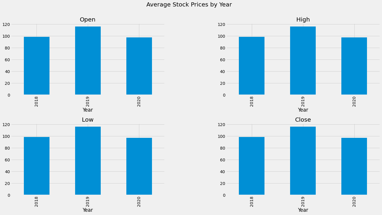
data['Year'] = data['Date/Time'].dt.year
data_grouped = data.groupby('Year').mean()

plt.subplots(figsize=(20, 10))
plt.subplots_adjust(hspace=0.4, wspace=0.4)

for i, col in enumerate(['Open', 'High', 'Low', 'Close']):
    plt.subplot(2, 2, i+1)
    data_grouped[col].plot.bar()
    plt.title(col)
    plt.suptitle('Average Stock Prices by Year', fontsize=20)

plt.show()
Tạo Bộ Dữ Liệu Huấn Luyện và Kiểm Tra
Chúng ta sẽ chia dữ liệu thành hai phần: một phần dùng để huấn luyện mô hình và một phần dùng để kiểm tra mô hình. Dữ liệu sẽ được chuẩn hóa và chia thành các chuỗi thời gian.
dataset = data['Close'].values
training = int(np.ceil(len(dataset) * .95))
print(training)
from sklearn.preprocessing import MinMaxScaler

scaler = MinMaxScaler(feature_range=(0, 1))
dataset = dataset.reshape(-1, 1)
scaled_data = scaler.fit_transform(dataset)

train_data = scaled_data[0:int(training), :]
# prepare feature and labels
x_train = []
y_train = []

for i in range(60, len(train_data)):
	x_train.append(train_data[i-60:i, 0])
	y_train.append(train_data[i, 0])

x_train, y_train = np.array(x_train), np.array(y_train)
x_train = np.reshape(x_train, (x_train.shape[0], x_train.shape[1], 1))
Xây Dựng Mô Hình LSTM
Mô hình LSTM sẽ giúp chúng ta dự đoán giá cổ phiếu dựa trên dữ liệu lịch sử. Mô hình sẽ có hai lớp LSTM, một lớp Dense, và một lớp Dropout.
model = keras.models.Sequential()
model.add(keras.layers.LSTM(units=64,
							return_sequences=True,
							input_shape=(x_train.shape[1], 1)))
model.add(keras.layers.LSTM(units=64))
model.add(keras.layers.Dense(32))
model.add(keras.layers.Dropout(0.5))
model.add(keras.layers.Dense(1))
model.summary
model.compile(optimizer='adam',
			loss='mean_squared_error')
history = model.fit(x_train,
					y_train,
					epochs=10)
Đánh Giá Mô Hình
Chúng ta sẽ đánh giá mô hình bằng cách sử dụng sai số bình phương trung bình (MSE) và sai số bình phương trung bình căn (RMSE).
mse = np.mean(((predictions - y_test) ** 2))
rmse = np.sqrt(mse)
print("MSE:", mse)
print("RMSE:", rmse)
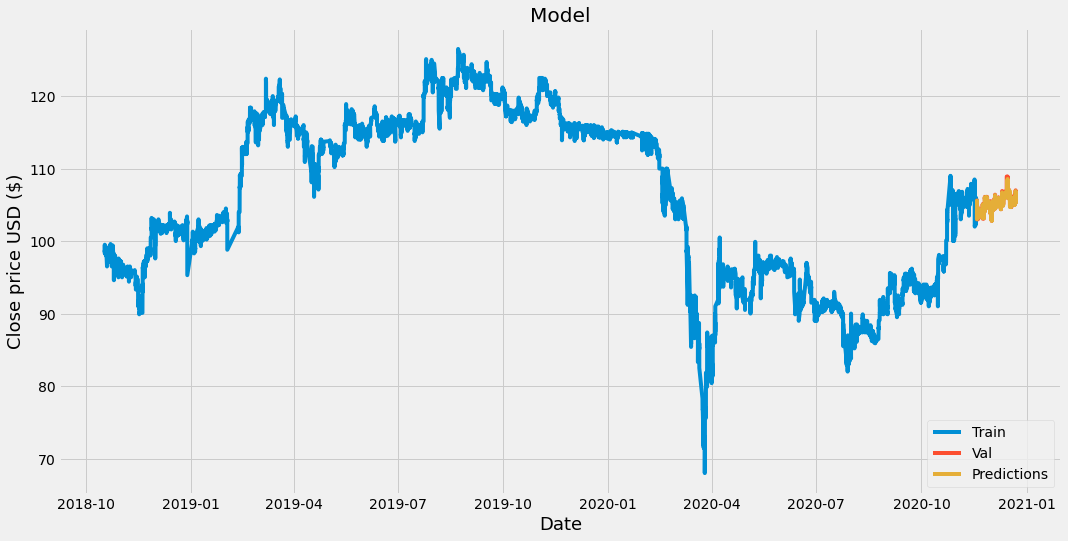
Dự đoán giá cổ phiếu trong tương lai
train = data[:training]
valid = data[training:]
valid['Predictions'] = predictions
#Visualize the data
plt.figure(figsize=(16,8))
plt.title('Model')
plt.xlabel('Date', fontsize=18)
plt.ylabel('Close price USD ($)', fontsize=18)
plt.plot(train['Date/Time'], train['Close'])
plt.plot(valid['Date/Time'], valid['Close'])
plt.plot(valid['Date/Time'], valid['Predictions'])
plt.legend(['Train', 'Val', 'Predictions'], loc='lower right')
plt.show()
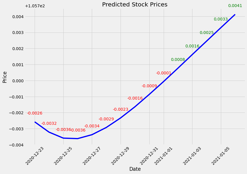
          Date       Price    Change
0   2020-12-23  105.697426 -0.002574
1   2020-12-24  105.696785 -0.003215
2   2020-12-25  105.696411 -0.003589
3   2020-12-26  105.696381 -0.003619
4   2020-12-27  105.696625 -0.003375
5   2020-12-28  105.697075 -0.002925
6   2020-12-29  105.697670 -0.002330
7   2020-12-30  105.698364 -0.001636
8   2020-12-31  105.699135 -0.000865
9   2021-01-01  105.699936 -0.000064
10  2021-01-02  105.700768  0.000768
11  2021-01-03  105.701614  0.001614
12  2021-01-04  105.702454  0.002454
13  2021-01-05  105.703293  0.003293
14  2021-01-06  105.704124  0.004124
Bạn có thể tìm full code ở đây Colab